Glossary

Task Type

In engineering practice, common machine learning modeling tasks include regression, classification and clustering。

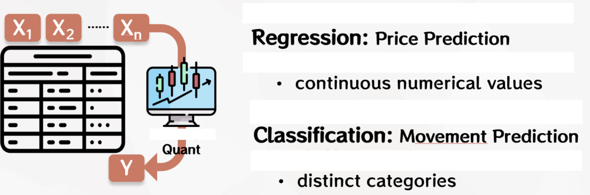
• Regression: Aims to predict continuous values, such as house price forecasts or sales volume forecasts.

• Classification: Aim to divide data into different categories, such as spam detection or disease diagnosis.

• Clustering: Aim to group data into similar groups to help uncover underlying structures in the data, such as market segmentation or customer group analysis. It is important to emphasize that we may not know how many market segments and customer groups exist before modeling.

Regression and classification tasks are also known as supervised learning, and users are required to label each data sample in modeling, so that the algorithm is supervised and guided in the learning process. This guidance helps algorithms understand the relationship between inputs and outputs and make accurate predictions or classifications when faced with new, previously unseen data.

Clustering tasks are called unsupervised learning because in such tasks, the model does not rely on pre-labeled or known outputs to learn. Instead, algorithms need to discover underlying structures or patterns in the data, grouping data samples into similar groups without needing to know the labels of those categories in advance.

In engineering practice, tasks with supervised learning are generally more common because it applies to many real-world problems and labeled data is easier to access and use, so the platform currently supports only two modeling tasks, regression and classification.

Whether the modeling task is regression or classification needs to be defined by the user according to the actual situation. For example, in the quantitative investment scenario, we can predict the value of the stock price tomorrow, so that the label is a continuous value, which is the regression task. We can also choose to predict the direction of the rise and fall of the stock price tomorrow, so that the label is the two categories of rise and fall, which is the binary task. Of course, we can also subdivide into more categories according to the different degrees of rise and fall, which is the multi-classification task.

Modeling Mode

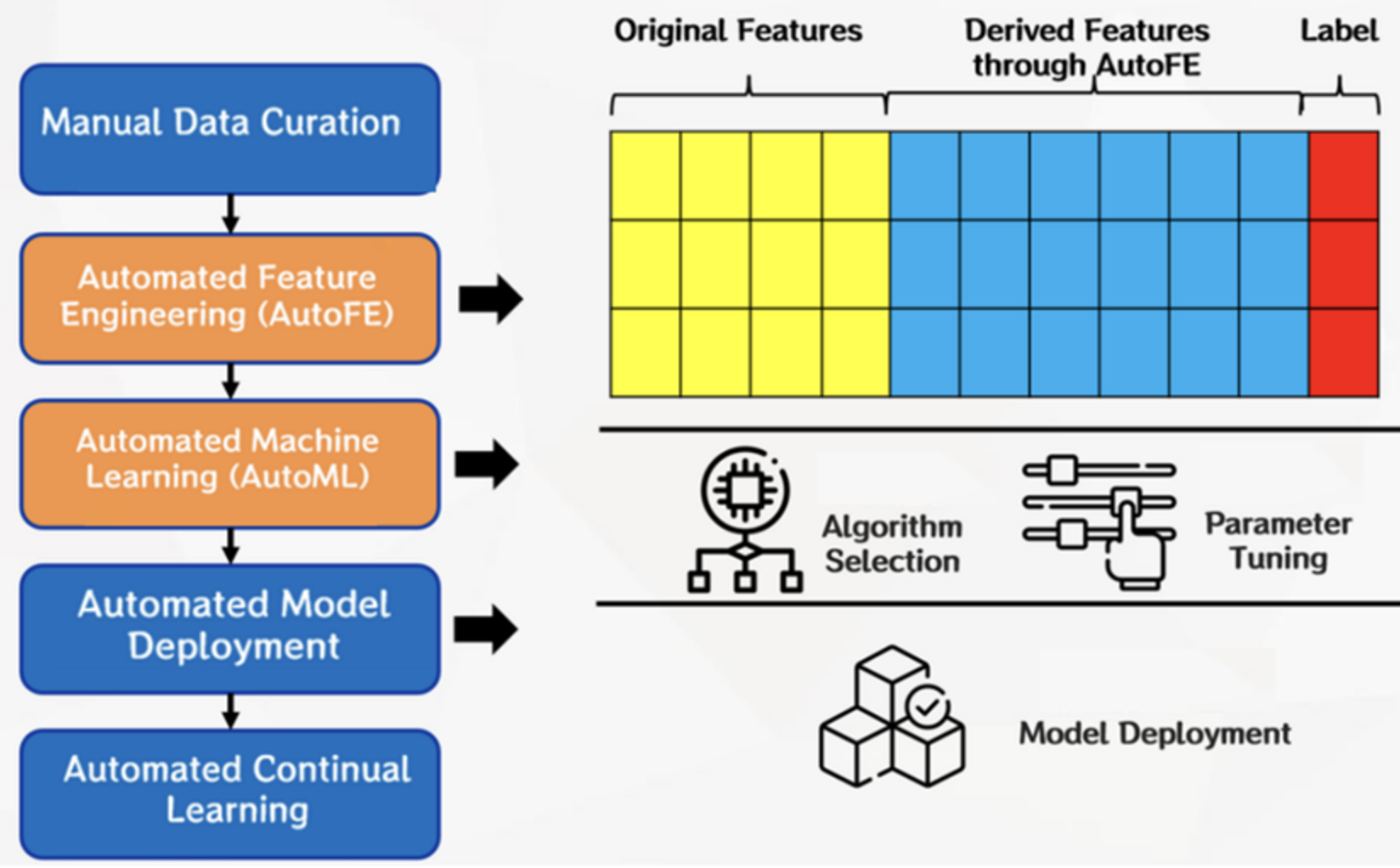
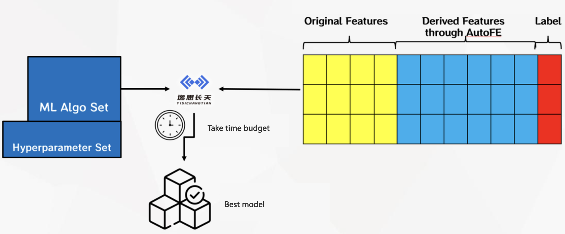
After the user manually collates the data set after uploading, and configures and starts the modeling task, the platform defaults to automatic feature engineering (AutoFE) and then automatic machine learning (AutoML) in the background. You can also deselect this option in Advanced configuration.

In AutoFE, the platform will build and efficiently explore the feature space according to the original features and platform operators, so as to automatically generate and derive features, build the feature group with the greatest common gain, and provide users with more new angles and new methods to interpret data.

In AutoML, the platform will automatically select algorithms and tune hyperparameters according to upstream features and labels. If the AutoFE process is performed upstream, the feature here contains both the original feature and the AUTOFE-derived feature, otherwise only the original feature is included. We recommend that users use both AutoFE and AutoML for better modeling results.

AutoFE

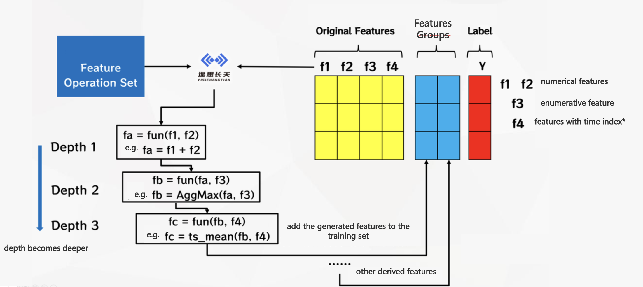
The Chinese name of AutoFE is Automated Feature Engineering. This platform has a built-in automatic feature engineering search algorithm developed by YiSiChangTian, which will build and efficiently explore the feature space according to the original features and operators of the data set uploaded by users (see AutoFE operator), and gradually generate and derive features.

In the process of feature generation, there is a certain probability that deeper feature derivation will be carried out on the basis of shallow derivative features, and deeper data rules can be mined by simultaneously optimizing the direction of each feature representation. Finally, the platform will explore the feature group with the greatest common gain. These advanced features have explicit formulas and better interpretability, providing users with a new Angle and a new method to interpret data.

In the field of automated feature engineering technology, there are still challenges that feature exploration space is huge and it is difficult to control the exploration process, so our team designed and balanced the two modes of adoption and exploration.

In the adoption mode, AutoFE will search according to the optimal path previously explored, without considering those sub-optimal paths, which has the advantage of speeding up the convergence of the search process, but it may also miss the feature construction results that are better in the long term because of the "short-term profit".

In the exploration mode, the opposite is true, AutoFE will diverge to generate more paths, and then further divergent search in some of the better performing paths. This has the advantage of exploring more possibilities, but it also consumes a lot of time.

tip

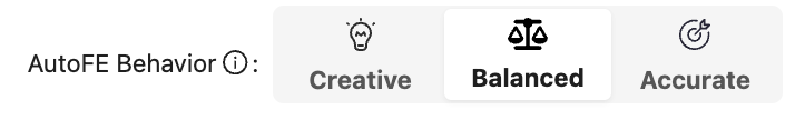
Because these two ways are you have me, I have you. So the platform gives users three options: be more creative, be more balanced and be more precise. More precision and more creativity correspond to "more adoption, less exploration" and "more exploration, less adoption" respectively, and more balance is a compromise between the two, and our default configuration also recommends a more balanced mode.

When creating a task, the user can select Advanced Settings to set it through the option of AutoFE Style, as shown in the following figure:

Added Deep Feature Search option to the general configuration section of the modeling task, which is checked by default. This means that we do a deeper nested search for features, which also takes more time. Otherwise, it will be nested shallow, such as: nested one or two layers. If users feel that overly complex features are not interpretable, you can uncheck them here.

AutoML

The Chinese name for AutoML is Automated Machine Learning. This platform has a built-in automatic machine learning algorithm developed by YiSiChangTian, which will search for the optimal machine learning model under the given time budget of the user according to the upstream data set, the machine learning algorithm and its corresponding hyperparameter set.

Random Seed

The random seed is a starting point or seed value used to initialize a random number generator, usually a positive integer. In machine learning and statistical modeling, many algorithms and models use randomness, such as random number generators for data splitting, weight initialization, or sample sampling. The generation of these random numbers is based on initial seed values.

The random seed can control the randomness of the model in different runs, so that the experimental results can be reproduced (with other configurations unchanged). If you do not set random seeds, the random numbers generated at each run may be different, resulting in different results each time you run the model. After the random seed is set, even if the model or algorithm is re-run, as long as the seed value is the same, the generated random number sequence will remain consistent, thus ensuring the repeatability of the results.

Maintaining reproducibility of results is important for experimental replication, model evaluation, and debugging. Therefore, it is a common practice to set random seeds during modeling to ensure consistency and reproducibility of results.

Verification Set Segmentation

Validation set segmentation is used to evaluate the performance and generalization ability of the model. In the initial stage of modeling, the platform will divide the data set into two parts: training set and verification set according to the segmentation method and segmentation ratio set by the user. In general, the proportion of the training set should be larger to allow the model to gain more information during the training phase.

The platform will use the training set to train the model, but the final model is evaluated against a new and unseen validation set, and the score of the modeling results seen by the user in the platform page is based on the results of the validation set.

Validation set segmentation will help improve the generalization ability of the model, that is, the ability of the model to adapt to new data. If the model performs well on the training set but poorly on the validation set, there may be an overfitting problem, that is, the model is over-adapted to the training data and does not generalize well to the new data.

The platform supports the following common verification set segmentation methods:

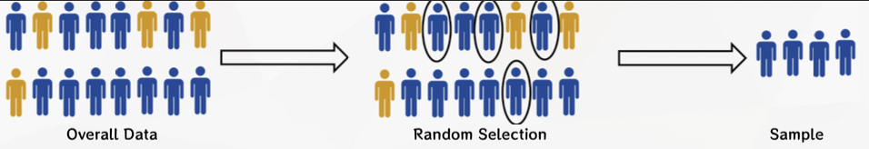
• Random sampling: Samples are randomly drawn from the entire data set as validation sets and training sets, without specific distribution requirements.

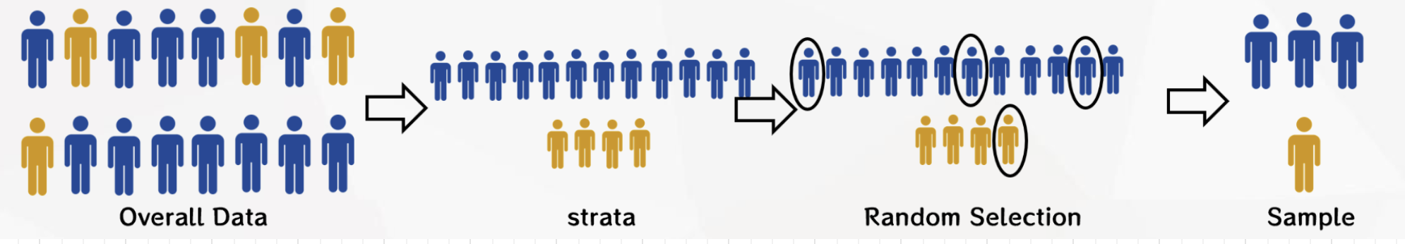
• Stratified sampling: A similar label distribution is maintained when the validation set and the training set are shred based on the distribution of labels or classes. This is especially useful in cases where the label categories are unbalanced to ensure that both the training set and the validation set contain representative samples of each category.

• Time segmentation: In the time series data, the verification set and the training set are segmented according to the time order (to prevent disturbing the time order and affecting the timing feature construction). This is a common segmentation method for time-dependent data sets, such as stock data, weather data, etc.

• Manual segmentation: The training set and validation set are segmented by the user manually uploading the data set file.

In engineering practice, when the distribution of sample labels for classification tasks is often not balanced, such as in the financial field, the incidence of fraudulent transactions is often relatively low. At this time, if the data set is still divided by random sampling, there is a large probability that there are no samples of fraudulent transactions in the verification set, thus greatly reducing the validity of the scores evaluated by the verification set.

In this case, stratified sampling will avoid the above situation. By first stratifying the aggregate data according to the sample label, and then sampling each type of label separately in proportion, it is possible to ensure that the training and verification sets have sufficient samples of fraudulent transactions.

tip

When you chooses traditional classical machine learning, the verification set segmentation method supports: stratified sampling, random sampling and manual segmentation.

When you chooses time series machine learning, the verification set segmentation method supports: time segmentation and manual segmentation.

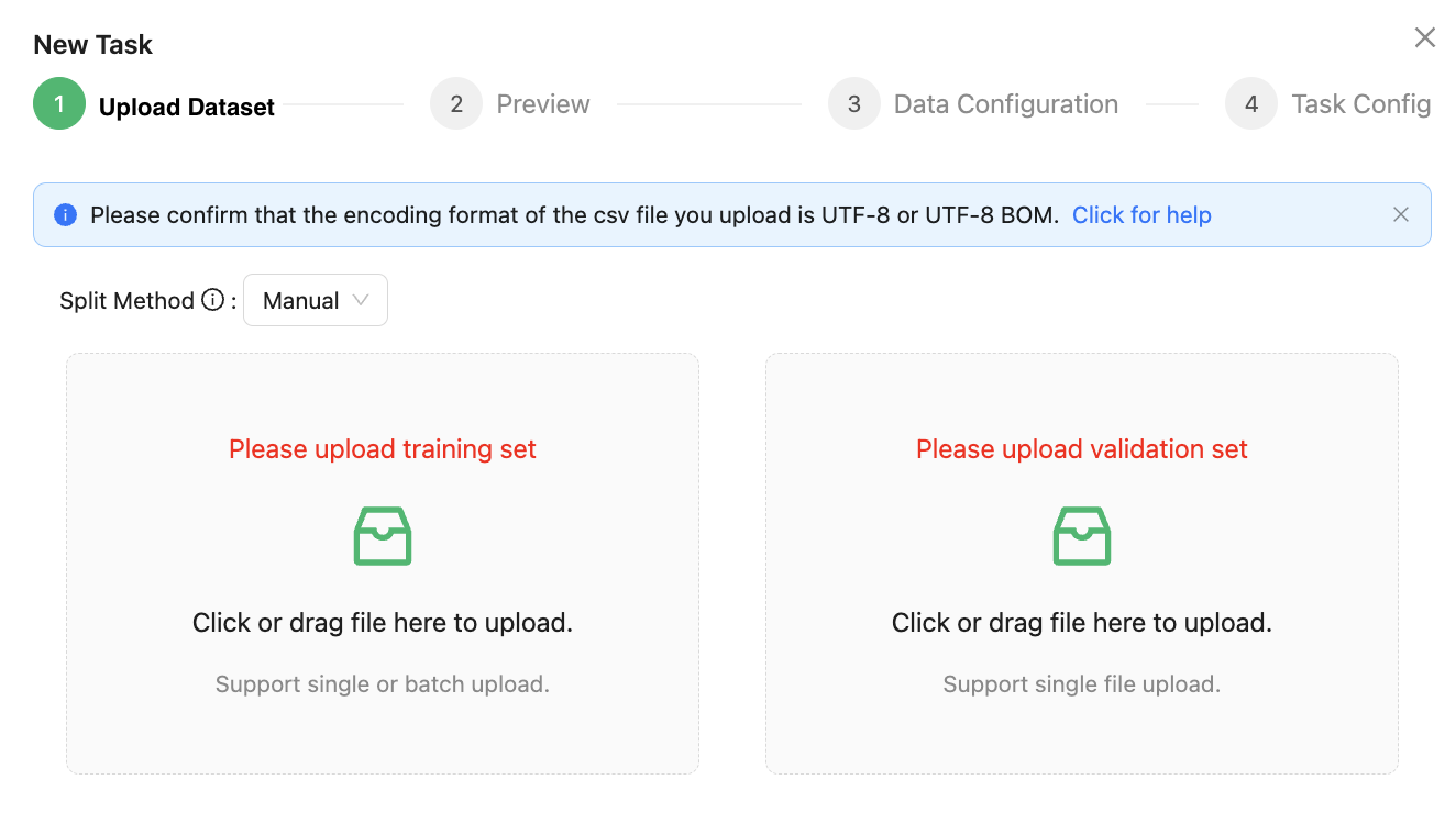
Other than manual segmentation, validation set segmentation has a certain randomness, and sometimes it is difficult to segment the data set according to the specified requirements. The user can choose to manually split the training set and the verification set. In this case, the two data files of the training set and the verification set need to be uploaded separately, as shown below:

Time Series

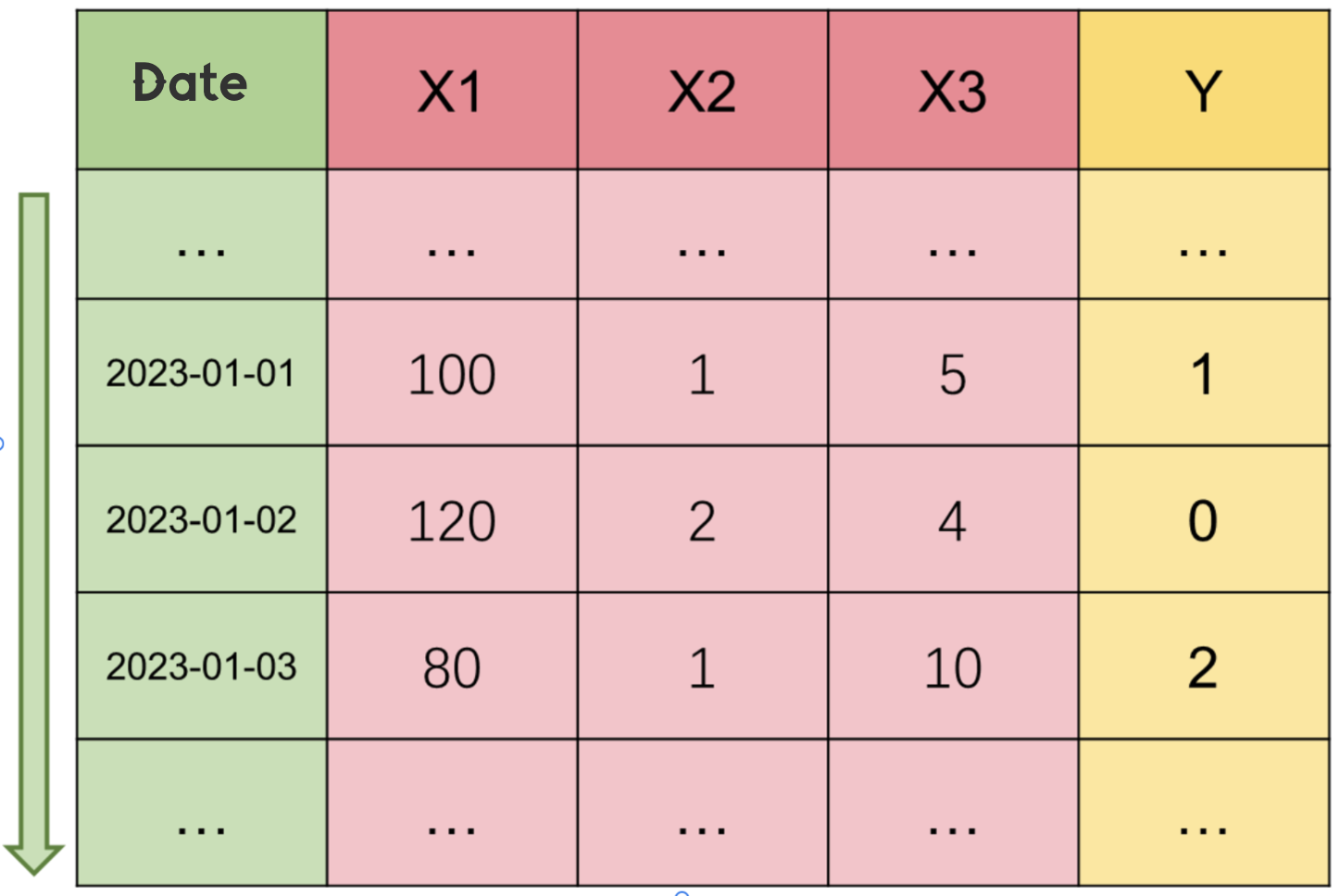
As the name suggests, time series is a collection of data points arranged in chronological order. These data points are usually collected or observed at equally spaced time intervals. Time series can be various types of data, such as stock prices, temperature, sales data, sensor readings, etc. Such data is usually labeled with a time column, which can be sorted in ascending order by time.

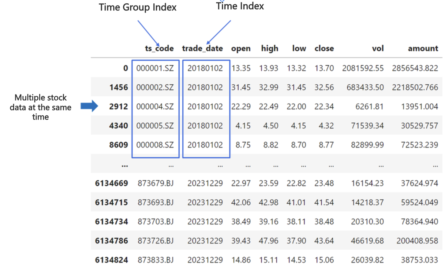
For some special time series data, there may also be time group identification to distinguish who produced the data at the same time, such as the characteristic data of multiple stocks at a time, or sensor data, and so on.

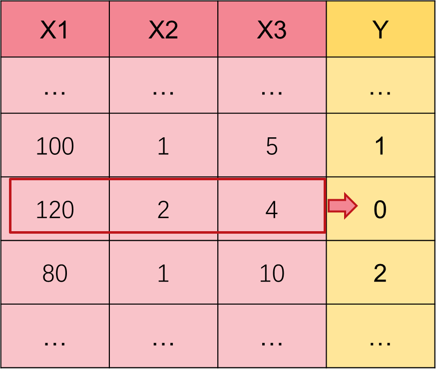
In traditional classical machine learning modeling tasks, we often use one or more features of a row of data (X1, X2, X3) to predict the Y label of this row, and we default that the information needed to predict Y is already contained in the features of this row.

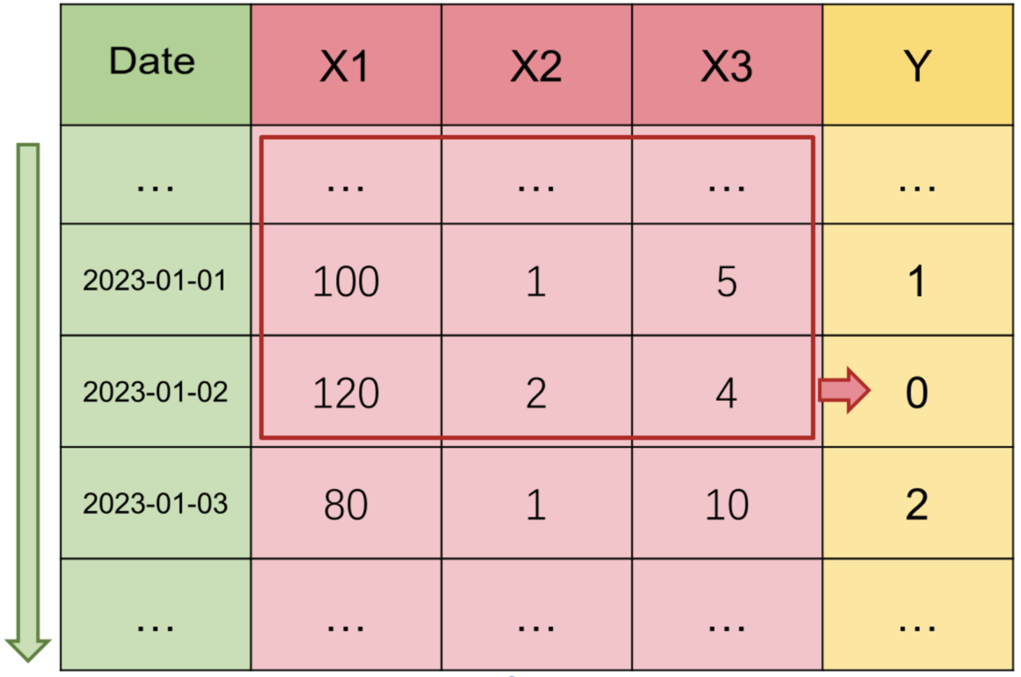
However, for the modeling scenario of time series, if we believe that there are certain patterns, trends and periodicity in the current time series, we should not only use the feature information of the current moment to predict Y during modeling, but also look back at the past feature information of the current moment to predict Y.

It should be emphasized here that although some data is the form of time series, since there is no historical law such as trend cycle, such modeling tasks do not belong to time series modeling tasks, such as lottery number prediction, obviously has nothing to do with past information. Therefore, whether a modeling task belongs to classical machine learning or time series machine learning needs you to judge for yourself, but obviously no time column index must not be a time series.

Then we refine the operation of time series machine learning, focusing on two issues:

tip

① How does a computer recognize time columns in different formats?

② How does the platform absorb historical feature information?

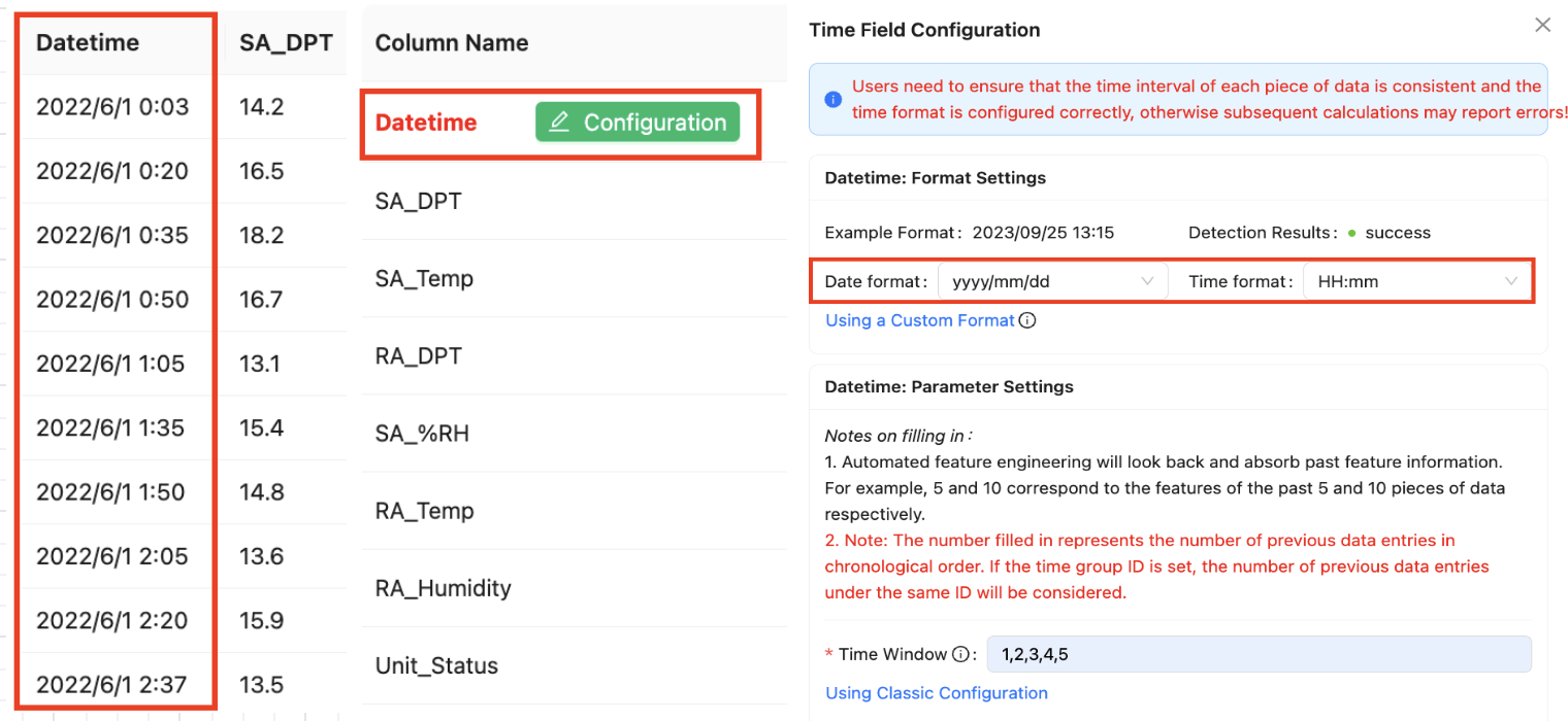
For the time column format, because it does have a high degree of flexibility, we will give it to the user to define, the user after uploading the data set, which column will be selected, and then there will be a configuration button for the user to configure.

Taking the daily frequency data of futures data in the financial field as an example, because its data is daily level, the user can select the date format when configuring, and here "2022/6/1" also meets the "yyyy/mm/dd" format. If your format is not this date performance, but "06/01/2022", it is the same as "YYYY-MM-DD". Then you can customize the value to "mm/dd/yyyy".

Here is a comparison table about time for your reference:

Format	Example
yyyy	year, e.g. 2023
mm	month, e.g. 12
dd	day, e.g. 01
HH	hour, e.g. 09
mm	minute, e.g. 30
ss	second, e.g. 10
SSS	millisecond, e.g. 125

info

The representation of time as letters must remain consistent, while the symbols used between different time granularities can be defined arbitrarily.

Then we look at how to absorb historical feature information, just introduced in the time series modeling data mentioned, to look back at the current moment of the past feature information to predict Y, then how much to look back, in fact, this needs to be based on the specific situation of the business.

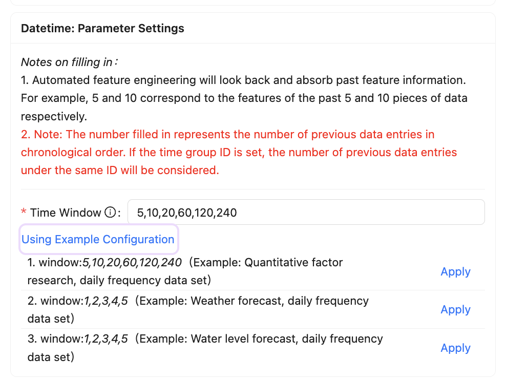
For example, in the stock volume and price data of financial investment, the data of the past 5 days and 10 days contain short-term market information, 20 days and 60 days are medium-term, 120 days and 240 days are long-term, and 240 days are also close to the trading days of a year in the stock market. However, for the water level prediction in the water conservancy scene, it may not be necessary to consider so many days, and the information of the past 5 looking Windows (1, 2, 3, 4, 5) is enough.

Therefore, we also open this configuration to the user to define, the user needs to enter a series of continuously increasing numbers to represent the different time Windows, separated by English commas. The automated feature engineering will then look back and absorb the past feature information, such as 5,10 corresponding to the features of the past 5 and 10 data respectively.

Note that the numbers you fill in represent the number of previous data entries in chronological order; if a time group identifier is set, the number of previous data entries under the same identifier is considered.

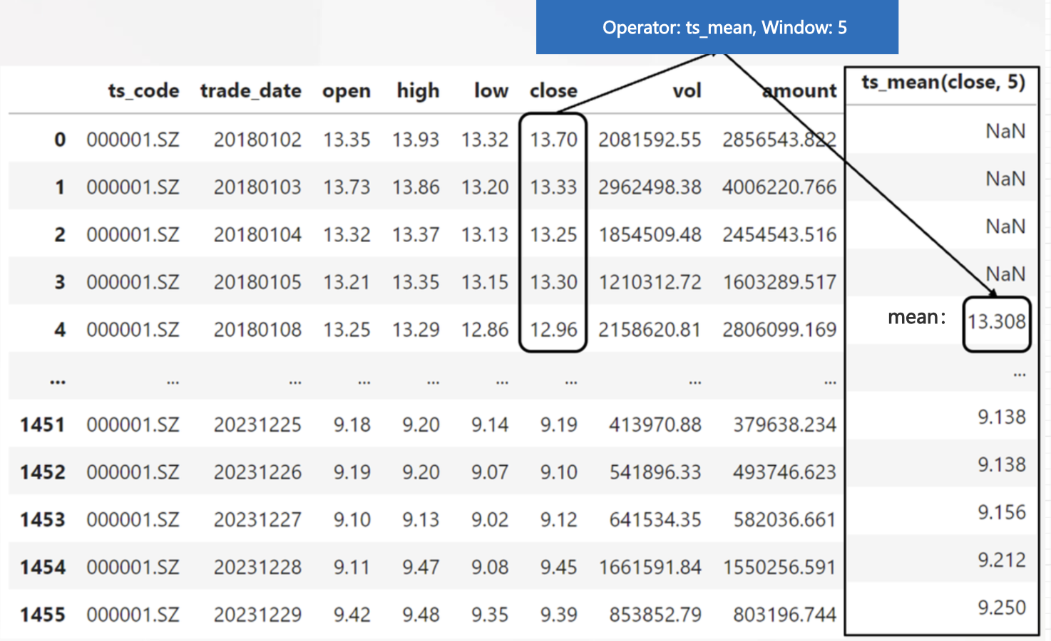
For example, we might search for the average closing price of the last 5 days: ts_mean(close, 5), and combine it with the window to generate the possibility: ts_mean(close, 10), ts_mean(close, 20), etc., and deeper nesting of features will be performed as the search depth increases (for more operators, see the time series operators section in the AutoFE Operator).

In addition, in the time series data modeling, in the face of the ever-changing external environment, only the method of proportional segmentation according to time is supported in the verification set segmentation, so as to prevent the time interval discontinuity of data caused by random sampling and hierarchical sampling. This method can effectively deal with the data dynamics caused by time changes, allowing the model to be trained and verified in different time periods, and better reflect the changes in the real environment.

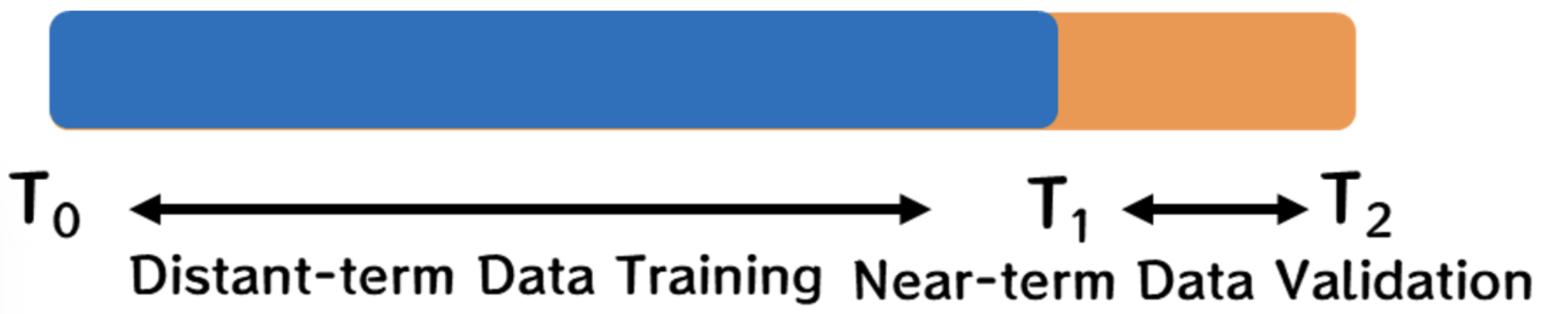
For example, in the scenario of predicting whether the user is overdue in the future for credit risk control, engineers generally arrange the data in ascending order according to time, and then select a certain time point, divide the data into two parts: long-term and recent, and then use long-term data training and recent data verification to evaluate whether a certain behavior law in the past is still applicable in the current.

In order to be compatible with the segmentation ratio parameters of other modes, the segmentation ratio of this platform for the time segmentation mode is also in the form of 0 to 1 decimal input, the default is 0.25, that is, 75% of the forward data is used for training, 25% of the recent data is used for forecasting. Users can manually adjust according to the actual situation.

Resampling

In machine learning classification tasks, the problem of unbalanced data set label samples often occurs, although we can use methods such as roc_auc (see: Model Evaluation Metrics) to reasonably evaluate the modeling results under sample imbalance, but in the model training will absorb more data information of label samples, so we can still have a lot of options to adjust the data set distribution, generally including up-sampling and down-sampling methods, they are collectively referred to as oversampling.

tip

Upsampling: Balance different categories of samples in the dataset by increasing the number of samples, such as copying, SMOTE synthesis, etc.

Downsampling: Balancing a dataset by reducing the number of samples in a category, such as random or selective deletion.

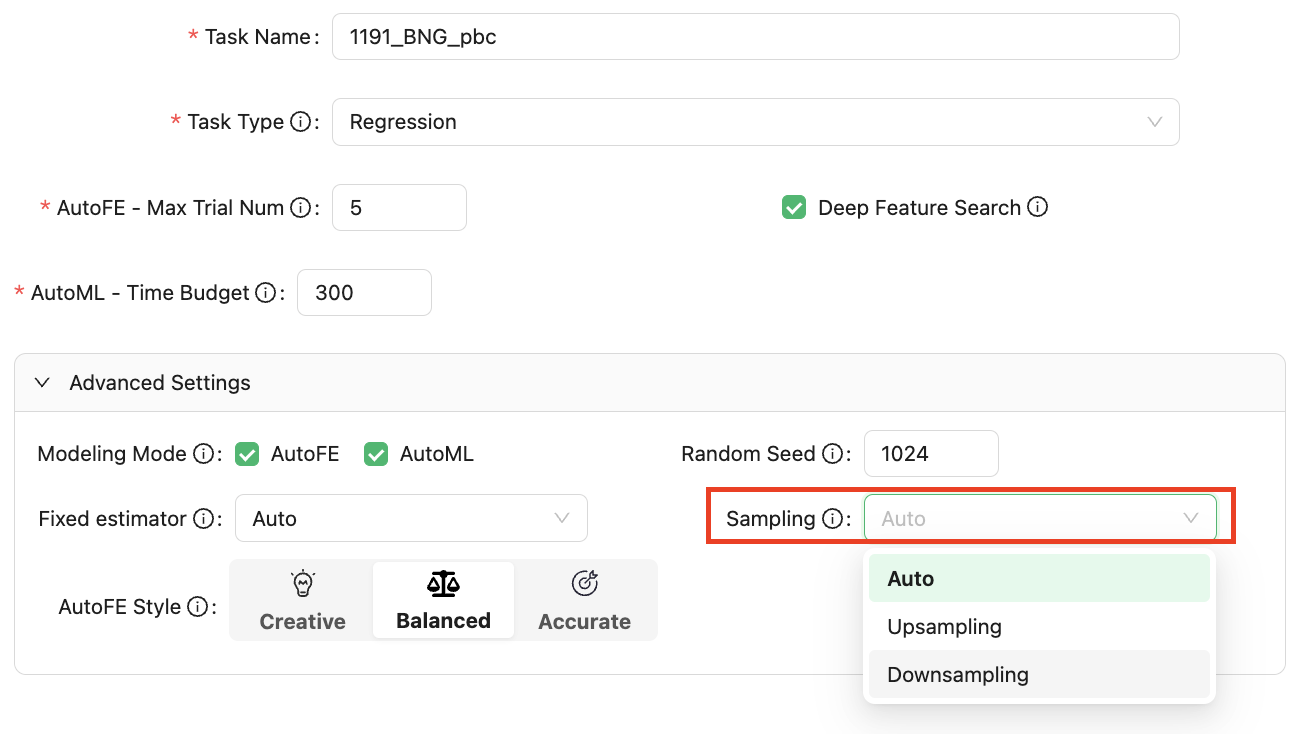
Because downsampling may lose the valid information of the sample, the result of the upsampling synthesis method is also untrue data, and the criteria for different modeling tasks are different. At present, users can select three sampling modes in the advanced Settings: automatic, up-sampling, and down-sampling. The default is automatic, as shown in the following figure:

tip

If the current task type is a regression task, no sampling is performed. If the current task type is a classification task, and most classification labels are unbalanced, for example, some labels have a 100:10 ratio of True to False.

① If upsampling is selected, the data corresponding to the False label is expanded to 100 by replication, and becomes 100:100.

② If downsampling is selected, the data corresponding to the True label is sampled 10 times and becomes 10:10.

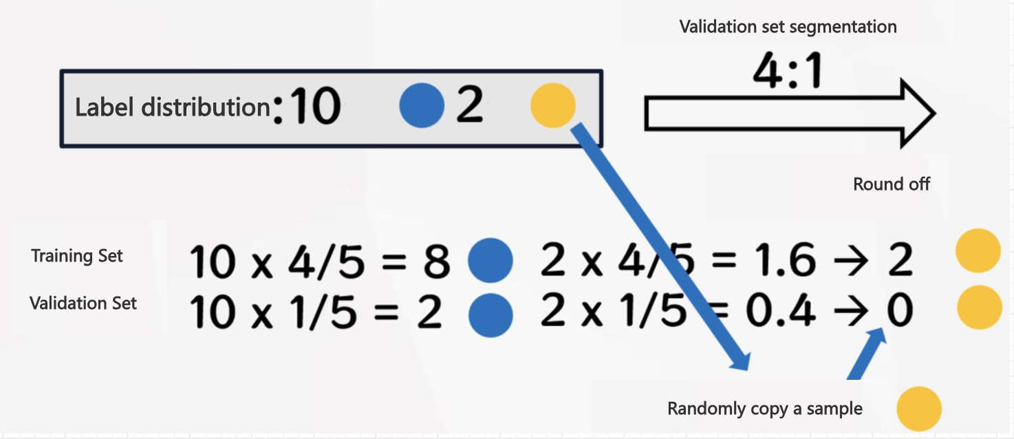
③ If automatic is selected, the sampling operation is not triggered unless the data corresponding to the minimum category is very small, and the number of data after multiplying the verification set segmentation ratio is less than one. In this case, the data of the minimum category is copied to meet the condition that there are integer data after segmentation.

Unless there are too few labeled samples in the verification set due to too few data point samples in the user's data set after the segmentation of the data set, the resampling mechanism of the platform will be triggered, and the process will copy the user's samples of this category, so that the verification set can have at least one sample of this category. The final result of the model may be slightly affected.

In this case, the platform will prompt the modeling result that triggers resampling. In this case, it is recommended to address the problem in two ways:

tip

Method 1: The optimal solution is that you can collect enough data for training.

Method 2: You can adjust the validation set separation ratio in the advanced Settings so that at least one sample can be assigned to the validation set.

When resampling is triggered at the same time, a "resampling" prompt will appear for the corresponding task in the modeling task column, as shown in the following figure: